A Krylov Approximation Method for Quantum Evolution

This post was originally published on Medium, and is being syndicated here.

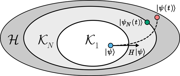
Laboratories around the world are in the race to develop increasingly accurate quantum devices. To carry out this successfully, it is necessary to compare quantum devices against classical devices. For this reason, it is important to have efficient classical algorithms to perform quantum simulations. Krylov-subspace methods approximate the exponential of a matrix on a vector. For quantum simulation, the mechanics of the approximation are the following. An initial state in a (possibly very) large Hilbert space is first mapped to an effective subspace, the Krylov subspace, that captures the most relevant features of the dynamics. Within this low-dimensional subspace, time evolution is (cheaply) computed. Finally, the evolved state is mapped back to the large Hilbert space. Besides quantum simulation, the method has other important applications like solving systems of ordinary differential equations ref, large-scale linear systems, finding the best dimension for PCA ref, and more.

Schematic of Krylov Approximation Method

The physics of Krylov-error: Loschmidt echo approach

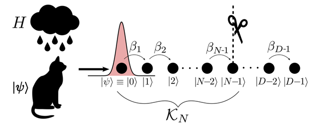
The evolution in the effective subspace is determined by a tridiagonal matrix; this type of system is equivalent to a tight-binding model with random hopping probabilities. The initial state starts at one end of the chain and starts to propagate throughout the sites. The approximation comes from cutting off the chain at one site. Now the error in the method is nothing but the Loschmidt echo between evolving forward with the full chain and backward with the cut version.

The dynamics of |ψ> under H, from the Lanczos Basis perspective, corresponds to the diffusion of an initial state |0> that is completely localized at the leftmost end of a virtual tight-binding chain.

This view of the problem makes it clear that the error will grow when the wave function starts to populate the site after the cut. The details of this analogy and how it is used to determine the error bound is discussed in our research paper https://arxiv.org/abs/2107.09805.

Error bounding and efficient iterations

One of the biggest problems with this type of method is the control of the error. After a short time, the error starts to grow exponentially. For the method to be useful one must restart the subspace when the error reaches a certain threshold. With this in mind, tight error estimation becomes crucial. If the bound overestimates the error one may end up doing a lot more iterations than needed and the method becomes inefficient.

The solution to the bounding problem

Taking inspiration from the analogy between the Krylov method and the tight-binding model presented above, one cheap and efficient way to estimate the error is to approximate the missing hopping amplitudes with the average of the previous ones. This leads to a tighter, almost perfect bound that translates to an optimal number of iterations (see figure).

Overestimation between different bounds and the real error vs the real error of a Krylov method. The black line is a classical bound proposed by Saad, the blue and green lines are the bound generated by approximating the last hopping coefficient and all the coefficients respectively.

Algorithm implementation and use example

We have developed a Python software package to support these Krylow simulations called PyKrylovSolver. You can install directly from GitHub by doing,

pip install git+https://github.com/emilianomfortes/krylovsolver/

The package enables the time evolution of state vectors for time independent Hamiltonians, building on the Qutip framework.

The function krylovsolve evolve the vector (“psi0”) under the action of a Hamiltonian (“H”), using a krylov approximation of dimension (“krylov-dim”) and a tolerance imposed by the user (“tolerance”). The output is either the state vector or the expectation values of supplied operators (“e_ops”), computed at each time in a list (“tlist”). The following example evolves a spin chain of 8 sites under a transverse Hamiltonian,

Contribute

You are most welcome to contribute to the development of the algorithm by forking the PyKrylov Solver repository and sending pull requests, or filing bug reports on the issues page. Any code contributions will be acknowledged in the upcoming contributors section in the documentation.

Citing

If you use our error bound approach for the Krylov approximation in your research, please cite the original paper available here.